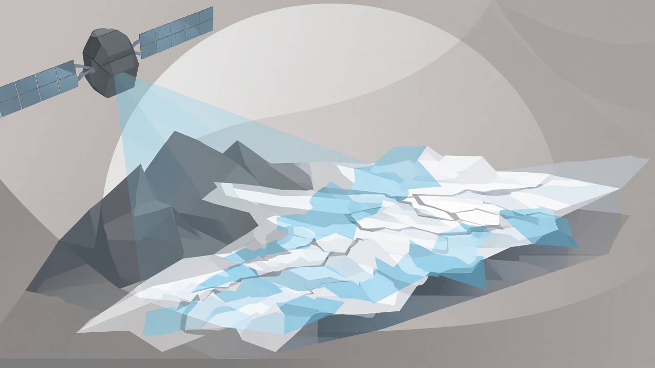
Glaciers are retreating worldwide, contributing to sea level rise and altering water supplies for hundreds of millions of people. Manual delineation from satellite imagery cannot keep pace with tens of thousands of ice bodies across polar and mountain regions. Deep learning segmentation on open optical and radar data now approaches expert delineation accuracy at global scale. GlaViTU (Glacier-VisionTransformer-U-Net), published in Nature Communications in January 2025 (doi:10.1038/s41467-024-54956-x), reports intersection-over-union scores above 0.85 on unseen images in most regions, with calibrated confidence maps and a benchmark covering nine percent of glaciers worldwide. Complementary frameworks such as DL4GAM monitor roughly nine hundred Alpine glaciers through 2023 using Sentinel-2 and elevation data. Readers interested in AI research for geospatial monitoring or popular AI tools for remote sensing workflows should understand how segmentation, validation stakes, and mass balance science connect before trusting automated ice loss headlines.
Why Manual Glacier Surveys Cannot Scale
Traditional glacier inventories require expert interpretation of satellite scenes, correction of semi-automated outlines, and revisits every few years, a process too slow for rapid climate feedback studies. The Randolph Glacier Inventory and regional updates depend on trained glaciologists who distinguish ice from rock, shadow, proglacial lakes, and debris-covered tongues where ice is hidden under surface rubble. High-Mountain Asia debris-rich glaciers remain especially labor-intensive. Climate models and water resource agencies need annual or seasonal change, not decadal snapshots. Automated mapping frees experts to validate edge cases rather than trace every polygon by hand.
Cloud cover, seasonal snow, and sensor differences complicate automation. A single misclassified snow patch can bias area trends. Multi-temporal strategies that select the best cloud-free observation per glacier, as in DL4GAM, reduce noise. Ensemble U-Net models with uncertainty quantification flag glaciers where predictions disagree, routing them to human review before inclusion in regional statistics.
Satellite Bands and Revisit Times
Operational AI glacier monitoring primarily uses Sentinel-2 multispectral imagery at ten-meter visible and near-infrared resolution with five-day revisit at the equator, supplemented by Landsat 8 and 9 at thirty-meter resolution and longer heritage records. Shortwave infrared bands help separate snow, ice, and water. Sentinel-1 synthetic aperture radar penetrates clouds and supports night observations, improving debris-rich and polar regions when fused with optical data in models like GlaViTU. Digital elevation models from TanDEM-X or regional LiDAR constrain ice surface slopes and help distinguish flat debris from ice underneath.
| Sensor | Resolution (typical) | AI monitoring use |
|---|---|---|
| Sentinel-2 optical | 10 m multispectral | Clean ice boundaries, snowline |
| Landsat 8/9 | 30 m multispectral | Long temporal baselines since 2013+ |
| Sentinel-1 SAR | 5 to 20 m radar | Cloudy regions, debris-rich ice |
| PlanetScope | 3 to 5 m (commercial) | High-frequency snow cover series |
Deep Learning Segmentation Workflows
Modern pipelines treat glacier mapping as semantic segmentation: convolutional or transformer U-Net architectures label each pixel as ice, non-ice, or optional debris classes on orthorectified tiles. GlaViTU combines convolutional encoders with Vision Transformer blocks and explores five multitemporal training strategies to generalize across regions and sensors. Reported IoU exceeds 0.90 in clean-ice-dominated areas, drops toward 0.75 in debris-rich High-Mountain Asia, and improves when SAR backscatter and coherence channels are added. Calibrated confidence scores accompany predictions so downstream users can mask low-certainty polygons.
DL4GAM applies U-Net ensembles with geographic cross-validation across the European Alps, estimating regional area change rates near negative 1.90 percent per year with uncertainty bands for 2015 to 2023, broadly consistent with prior expert assessments near negative 1.3 percent for 2003 to 2015. USGS Benchmark Glacier Project workflows use support vector machines and other classifiers on Sentinel-2, Landsat, and PlanetScope to derive snow-covered area, accumulation area ratio, and seasonal snow line time series from 2013 onward with overall accuracies between 92 and 98 percent compared to manual interpretations. Snow line altitude medians differ from manual delineation by about 31 meters, adequate for trend analysis but not replacement for stake measurements.
Ground-Truth Validation With Stakes and GPS
Satellite-derived area change validates against field stakes, GPS surveys, airborne photogrammetry, and independent expert digitizations before feeding mass balance or sea level assessments. Glaciologists drill ablation stakes, measure snow pits, and conduct geodetic mass balance flights on benchmark glaciers. AI outlines track geometric area and surface elevation changes when DEM differencing is available, but direct mass balance still requires density assumptions or gravimetry for total water equivalent loss. GlaViTU authors compare predicted boundaries to human expert variability, showing model distance deviations approach inter-expert spread in many tiles.
Validation design must avoid training and testing on adjacent tiles from the same glacier, which inflates scores. Geographic cross-validation held out entire mountain ranges in Alpine studies. Debris-covered tongues remain the largest error source; fusion of thermal, radar, and morphological features is an active AI research frontier. Until debris performance matches clean ice, regional totals for Himalayas or Andes should include explicit uncertainty envelopes.
Connecting Melt to Sea Level Projections
Area and elevation trends from AI monitoring feed regional glacier contribution estimates to sea level, combined with ice thickness models and climate forcing scenarios. Mountain glacier melt contributed noticeably to twentieth-century sea level rise and remains a significant term under RCP and SSP pathways, though ice sheets dominate long-term uncertainty. Automated inventories update glacier outlines used in global compilations such as the Randolph Glacier Inventory revisions and model initialization for hydropower stress studies in Asia and South America.
Antarctica and Greenland require ice sheet models with calving dynamics, not only outline segmentation. AI helps map surface melt zones and supraglacial lakes on ice sheets using similar remote sensing tools, but sea level projections integrate multiple processes. Himalayan water supply analyses pair area loss with downstream population exposure; AI acceleration makes seasonal runoff forecasts more timely for policy but does not remove political complexity around transboundary rivers.
Photogrammetry from repeat satellite stereo pairs and airborne campaigns provides elevation change independent of outline area alone. When AI segmentation pairs with DEM differencing, researchers estimate volume loss more directly than multiplying area trends by assumed thickness profiles. Sensor fusion workflows in GlaViTU demonstrate that adding Sentinel-1 coherence reduces confusion between stagnant ice and rock in shadowed valleys. Operational services for hydropower operators may eventually ingest near-real-time snowline products, but regulatory reporting still expects documented human sign-off on inventory revisions submitted to water authorities.
Frequently Asked Questions
Can AI replace glaciologists?
No. AI scales outline mapping and snow indicator time series; glaciologists design validation campaigns, interpret debris-covered errors, and connect ice loss to hydrology and hazards. Expert review remains essential for publication-quality inventories.
How accurate is GlaViTU?
The Nature Communications 2025 study reports IoU above 0.85 on most held-out regions, higher on clean ice and lower on debris-rich terrain. Performance is spatially variable; users should apply provided confidence masks.
What about Himalayan glaciers?
High-Mountain Asia is debris-rich and cloud-prone. Expect lower IoU than Alpine clean ice unless models fuse SAR and elevation data. Regional studies should report uncertainty explicitly rather than single point estimates.
Does Antarctica use the same models?
Continental ice sheets share remote sensing methods but require different process models for calving and basal melt. Segmentation tools map features such as melt ponds; sea level projections add ice sheet dynamics beyond area polygons.
Which resolution is enough?
Ten-meter Sentinel-2 resolves many valley glaciers; small cirque glaciers may need higher resolution or manual correction. Thirty-meter Landsat suffices for large ice bodies and long trends with coarser detail.
How often should outlines update?
Annual end-of-melt-season composites are common for area change. Snow indicators can update monthly or faster with PlanetScope or Sentinel-2 cloud-free stacks. Choose frequency based on hazard or water management needs, not model capability alone.
The Nature Communications GlaViTU paper released a benchmark covering nine percent of global glaciers with calibrated confidence outputs, giving downstream users a template for uncertainty-aware reporting. National mapping agencies can integrate such models into semi-automated production lines while reserving expert hours for debris-rich tiles flagged below IoU thresholds, balancing cost and scientific rigor.
Seasonal snow cover classifiers on Landsat and PlanetScope extend the same satellite stack beyond static outlines, producing accumulation area ratio time series that reveal whether melt seasons start earlier or end later than historical norms. Those indicators feed hydrological models for rivers fed by glacier and snow melt, linking remote sensing AI directly to downstream water allocation debates in arid regions.
Antarctica and Greenland ice sheets require ice sheet models with calving and basal melt processes that outline segmentation alone cannot supply. AI still assists by mapping supraglacial lakes and surface melt zones that precondition ice shelf collapse. Mountain glacier AI products should report versioned model weights and training regions so IPCC contributors can trace inventory updates in sea level chapter supplementary tables.
Manual stake measurements on benchmark glaciers remain the gold standard for annual mass balance at select sites. AI scaling fills gaps between those sites, letting regional totals update faster than decadal manual inventory cycles. Users exporting shapefiles from GlaViTU or DL4GAM should preserve confidence bands and sensor dates in attribute tables so downstream hydrological models propagate uncertainty rather than treating every polygon as equally reliable.
The Cryosphere journal's 2025 automated snow cover workflow reports median snow line altitude differences near 31 meters versus manual delineation across Landsat, Sentinel-2, and PlanetScope products. That accuracy supports seasonal melt indicators but not glacier thickness alone. Combining area loss from GlaViTU with geodetic mass balance flights on benchmark glaciers remains the recommended path for IPCC-style mass loss reporting.
High-Mountain Asia debris-covered glaciers remain the hardest test for global models: IoU can drop toward 0.75 in GlaViTU evaluations while clean-ice regions exceed 0.90. Adding Sentinel-1 backscatter and coherence channels improves performance where optical sensors fail, but no single model eliminates field validation on debris-rich termini feeding major Asian rivers.