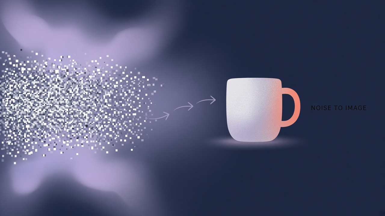
You type "a ceramic mug on a wooden desk, morning light" into an AI image generator and seconds later receive a sharp photograph that never existed. Under the hood, most modern image and video tools rely on diffusion models. Diffusion models explained in plain language: the system learns to reverse a gradual corruption process, starting from pure noise and removing a little randomness at each step until structure, color, and detail match your prompt. The same family of models powers inpainting, style transfer pipelines, and many AI code assistants that render UI mockups or diagram assets from text descriptions.
How Does Noise Become an Image?
A diffusion model treats image generation as the reverse of slowly adding Gaussian noise until a photo becomes static; at inference time the model predicts and subtracts noise step by step until a recognizable picture emerges. Think of a clear photograph fading into TV snow across hundreds of synthetic corruption stages. Training teaches a neural network to estimate the noise that was added at each stage. At generation time you begin with random noise and ask the network, "What noise should I remove here?" repeating that question for dozens or hundreds of steps.
The forward process (adding noise) is mathematically simple and does not require learning. The reverse process (denoising) is hard, which is why large U-Net or transformer backbones learn noise predictions conditioned on text embeddings from a separate encoder. Latent diffusion compresses pixels into a smaller latent space before denoising, which is why Stable Diffusion class tools run on consumer GPUs while full-resolution pixel diffusion remains research-heavy and expensive.
Forward and reverse intuition
Picture a stack of blurry versions of the same photo, each blurrier than the last until only noise remains. Diffusion training shows the model pairs of (slightly noisy image, exact noise added). The model learns a function that maps noisy latents plus timestep plus text prompt to a noise estimate. Sampling walks backward through timesteps from high noise to low noise. Early steps establish global layout and color; late steps refine edges, textures, and fine detail.
What Happens During Training vs Inference Sampling?
Training randomly picks a timestep, adds matching noise to real images from a dataset, and penalizes the model when its predicted noise differs from the ground truth; inference runs the learned denoiser repeatedly without access to original photos. Training data quality and caption alignment dominate what the model can render. Inference never sees training images directly. The model generalizes from learned denoising skill plus prompt conditioning.
Classifier-free guidance training drops text conditioning on some batches so the model learns both unconditional and conditional denoising. At inference, guidance scales the gap between conditional and unconditional noise predictions, sharpening prompt adherence at the cost of diversity and sometimes oversaturated colors. Samplers (DDIM, Euler, DPM++, and others) define how predicted noise translates into the next slightly cleaner latent. Different samplers trade step count against stability and artifact risk.
| Phase | Input | Output | Who pays compute |
|---|---|---|---|
| Training | Real images + captions | Denoiser weights | Lab or cloud GPU clusters |
| Inference sampling | Noise + prompt + seed | Final image or video frame | End user or API per generation |
| Fine-tuning (LoRA, DreamBooth) | Small custom image set | Style or subject adapter | Creator or enterprise team |
How Do Steps, Guidance, and Seed Control Output?
Sampling steps set how many denoising iterations run; classifier-free guidance scale pushes outputs toward the prompt; the seed fixes the initial noise tensor so identical settings reproduce the same image. More steps generally improve coherence up to a plateau, then waste GPU time. Many hosted tools expose 20 to 50 steps as defaults. Guidance scale around 7 to 9 is common for photorealistic prompts; lower values yield softer, more varied results. Seeds enable A/B testing of prompts while holding composition constant.
Negative prompts list attributes to suppress (blur, extra fingers, watermark text). They work by steering the unconditional branch during guided sampling. Schedulers map the continuous noise timeline into discrete step sizes. Fast schedulers reach acceptable quality at 15 to 25 steps; quality-focused workflows may use 40 or more on local GPUs. Batch size multiplies cost linearly: four variants at 30 steps equals four full sampling runs.
Reproducibility and variation
Identical seed, model version, sampler, steps, guidance, and prompt should reproduce the same latent trajectory on the same hardware and software stack. Model updates, different floating point kernels, or server-side optimizations can break strict reproducibility across releases. Creators who need variation fix the prompt and change only the seed to explore compositions while keeping lighting and layout similar.
How Do Image and Video Diffusion Differ?
Image diffusion denoises a single latent grid; video diffusion adds a temporal dimension, denoising stacks of frames jointly or predicting motion between keyframes so motion stays consistent across time. Early video tools generated short clips by applying image models frame by frame with flicker. Modern video diffusion models (Sora-class architectures, Stable Video Diffusion, Runway Gen-class pipelines) train on spatiotemporal volumes or use temporal attention so objects persist and camera motion stays smooth.
Image-to-video conditioning starts from one still and diffuses forward in time. Text-to-video models sample an entire latent video tensor from noise. Longer clips multiply memory and step cost roughly with frame count times resolution. Some products generate keyframes with image diffusion then interpolate with lighter models to save compute. Audio-driven avatar tools combine face diffusion with separate speech models.
| Modality | Typical latent shape | Main challenge |
|---|---|---|
| Still image | Height x width x channels | Anatomy, text in scene, prompt drift |
| Short video (2 to 6 s) | Frames x height x width | Temporal consistency, object identity |
| Inpainting / outpainting | Masked regions in latent space | Seamless blend at mask borders |
What Drives Compute Cost in Diffusion?
Diffusion cost scales with resolution, step count, model size, batch size, and whether generation runs in latent space or full pixels; video multiplies cost by frame count and temporal model depth. A 1024 pixel square image at 30 steps on a 2B parameter U-Net consumes far less than the same settings at 2048 pixels because attention and convolutions grow with pixel count. Hosted APIs price per image or per GPU second; heavy users should watch step defaults and resolution caps in tier tables.
Distilled models (fewer-step student networks) and turbo schedulers cut latency for preview workflows. Upscaling often runs as a second pass with a separate super-resolution model, doubling billable work for print-ready assets. Enterprise deployments amortize cost with dedicated GPUs, batch queuing, and caching popular prompts. Consumer apps hide complexity behind credit systems where one "HD" generation may equal several standard credits.
Cost levers creators control
- Lower output resolution until final approval, then upscale once.
- Reduce steps after finding a stable sampler for your style.
- Generate one seed at a time instead of large grids on every prompt tweak.
- Use inpainting on a base image instead of full rerolls for small edits.
- Pick models matched to task (photoreal vs illustration) to avoid wasted retries.
How Do Creators Evaluate Diffusion Tools?
Compare diffusion products on default step counts, maximum resolution, inpainting quality, model transparency, and whether pricing scales with steps or only with output size. A polished UI matters less than reproducible seeds, clear safety policy, and access to negative prompts or advanced sampler settings. Teams building marketing assets should test brand colors and product geometry on a fixed seed before committing credits to full campaigns.
Check license terms for commercial use, especially when base models train on scraped web images. Enterprise buyers should ask whether the vendor logs prompts, stores generations for retraining, and offers regional data residency. Developers integrating diffusion via API need webhook latency metrics, queue depth during peak hours, and documented model version strings so app updates do not silently change visual style.
Prompt engineering for diffusion
Effective prompts describe subject, medium, lighting, camera angle, and mood in concrete nouns rather than vague adjectives. Weight syntax (emphasis markers in some UIs) boosts important tokens. Reference artists or film stocks steer aesthetic bias baked into training data. Iteration beats one-shot perfection: adjust guidance before adding more steps, because high guidance with too few steps produces plastic textures, while many steps with low guidance yield dreamy but off-brief images.
Frequently Asked Questions
How do diffusion tools control artistic style?
Style control combines base model choice (trained aesthetic bias), LoRA or reference-image adapters, prompt keywords, and negative prompts. Some interfaces expose style presets that map to hidden prompt fragments or secondary model weights. IP-Adapter and similar methods inject reference image embeddings without full fine-tuning. Style strength sliders usually adjust adapter weight or guidance contribution.
What is inpainting in diffusion workflows?
Inpainting masks part of an image and runs partial denoising inside the mask while frozen regions stay fixed (or softly blended). Outpainting extends canvas beyond original borders. Both reuse the same denoiser with modified attention so new pixels match lighting and perspective of surrounding content. Product photo editors and generative fill features in creative suites rely on this pattern.
How do safety filters interact with diffusion sampling?
Safety stacks typically run classifiers on prompts before sampling and on outputs after decoding latents to pixels. Blocked prompts fail fast; flagged images may blur or reject. Filters do not change core diffusion math; they gate inputs and outputs. False positives affect legitimate medical, artistic, or educational prompts. Local open-weight models may omit hosted filters, shifting responsibility to the operator.
Why do diffusion images sometimes show extra fingers or warped text?
Hands and spelled text are underrepresented or ambiguous in training captions, so the denoiser lacks strong constraints for exact digit count or letter shapes. Higher step counts, inpainting retries on hands only, and models fine-tuned on anatomy help. Text in scenes remains unreliable unless specialized glyph-aware pipelines or post-processing OCR correction are used.
How do diffusion models compare to older GAN approaches?
GANs trained a generator against a discriminator in adversarial loops, often unstable and mode-collapsed on diverse prompts. Diffusion trades adversarial training for stepwise denoising, yielding broader prompt coverage and easier conditioning on text. GANs still appear in real-time face filters and some super-resolution paths where single-pass speed beats iterative sampling.
Conclusion
Diffusion models explained for creators and tool buyers: learn to denoise noise corrupted images during training, then at inference walk backward from random noise using text-conditioned noise predictions. Steps, guidance, and seed shape quality and reproducibility; video adds temporal modeling and steep compute growth. Understanding sampling cost helps you choose resolution, batch size, and hosted tier wisely. Evaluate AI image generator products on sampler options, safety transparency, inpainting quality, and whether pricing tracks steps and resolution honestly.