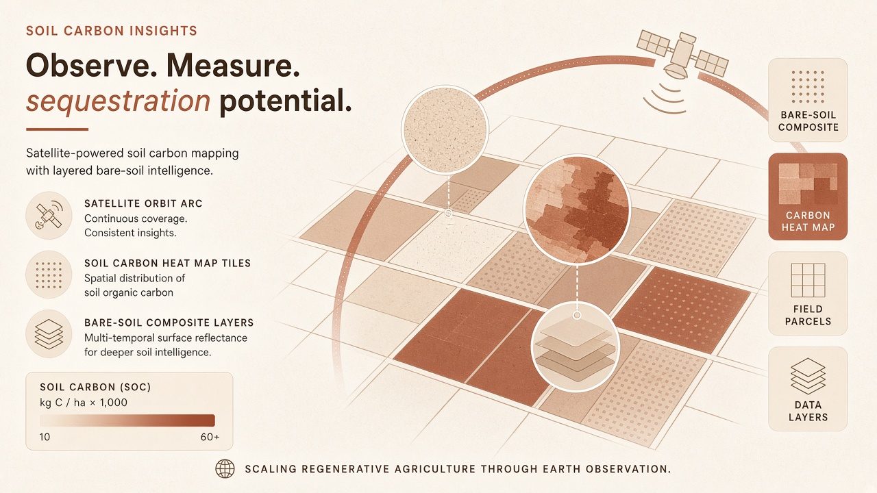
Carbon credit programs, regenerative agriculture contracts, and national greenhouse gas inventories all need soil organic carbon (SOC) estimates at field or regional scale. Traditional measurement relies on coring, dry combustion, or wet oxidation in labs, workflows that cost tens of dollars per sample and cannot cover every hectare each season. Remote sensing offers wall-to-wall coverage, but bare soil reflectance alone misleads when crop residue, moisture, and texture vary. Soil carbon measurement AI satellite combines Sentinel-2, Landsat 8 and 9, and Google Earth Engine (GEE) workflows with prior-data transformers and vision models to predict SOC where ground truth is limited.
Agronomists, carbon market developers, and land grant researchers all ask the same question: can a model trained on 174 cores generalize to a county? Product teams exploring AI chatbot interfaces for climate-smart agriculture should ground answers in reported R2, RMSE, and external validation splits, not marketing-grade certainty maps. More explainers live on the EliteAI.tools blog index.
What Soil Carbon Satellite AI Means in Plain Language
Soil carbon satellite AI is the use of machine learning on multispectral satellite time series, terrain derivatives, and sparse soil sample labels to predict soil organic carbon stocks or concentrations at pixel or parcel scale for monitoring, crediting, and research. Prediction is not laboratory replacement: satellite models interpolate patterns learned where cores exist and flag uncertainty where labels are absent; regulators and buyers still expect stratified ground truth for verification.
Modern pipelines pull Sentinel-2 red-edge and shortwave infrared bands sensitive to surface organic matter signals, harmonize Landsat 8 and 9 archives on GEE for longer baselines, and fuse climate, soil survey, and topographic covariates. Tabular foundation models like TabPFN excel when sample counts stay in the hundreds, while SSL-SoilNet vision transformers learn spatial context from unlabeled imagery before fine-tuning on labeled pixels.
| Input layer | SOC relevance | Typical source |
|---|---|---|
| Multispectral reflectance | Surface organic matter, residue, moisture confounds | Sentinel-2, Landsat 8/9 on GEE |
| Terrain and wetness | Deposition, erosion, drainage effects on SOC | DEM derivatives, flow accumulation |
| Soil survey polygons | Texture and taxonomy priors | SSURGO, WRB, national soil grids |
| Ground truth cores | Training labels, verification anchors | Field campaigns, dry combustion labs |
How the Soil Carbon Satellite Pipeline Works
A soil carbon satellite pipeline collects harmonized imagery and covariates on GEE or local stacks, aligns sparse core locations to pixel values, trains tabular or vision models with spatial cross-validation, exports SOC prediction maps with uncertainty bands, and reserves held-out cores for external validation before crediting or publication. Spatial honesty matters: random train-test splits inflate R2 when neighboring pixels share geology.
TabPFN plus Sentinel-2 for small sample regimes
TabPFN prior-data fitted networks paired with Sentinel-2 features report median hold-out performance around R2 of 0.78 and RMSE of 1.90 (units as reported in the source study, typically percent SOC or tonnes per hectare depending on label definition) on datasets with as few as N equals 174 ground samples. TabPFN targets small tabular problems where deep networks overfit; it ingests engineered spectral indices, texture class dummies, and elevation without extensive hyperparameter search. Small N success does not guarantee transfer to counties with different parent material unless new cores anchor predictions.
SSL-SoilNet vision transformers
SSL-SoilNet applies self-supervised learning with Vision Transformer (ViT) backbones on unlabeled soil and land surface imagery before fine-tuning on labeled SOC pixels. Pretraining captures spatial textures and seasonal vegetation dynamics that tabular-only models miss when crop cover masks bare soil signals. Transformer approaches demand GPU budget and careful masking of cultivated periods when residue cover dominates reflectance without deep SOC change.
Landsat 8 and 9 harmonization on Google Earth Engine
Landsat 8 and 9 surface reflectance collections on Google Earth Engine extend temporal depth before Sentinel-2 availability and fill gaps where cloud cover frustrates optical continuity. Harmonization routines align band responses across sensors so decade-scale trends in surface organic matter proxies remain comparable. GEE exports enable regional SOC dashboards without local raster storage, though large exports hit quota limits requiring tiled workflows.
Uncertainty quantification and P50 reporting
Responsible SOC maps report median predictions (P50) alongside prediction intervals from ensemble spread or quantile regression. TabPFN studies emphasizing P50 R2 of 0.78 communicate central tendency fit; credit protocols may require P95 conservative stocks so buyers are not exposed to optimistic means alone. Uncertainty layers should enlarge in sand hills and peat edges where training cores are sparse.
Verification sampling design
Model-first maps still need stratified verification cores each crediting period. Adaptive sampling can target high-variance pixels the model flags, reducing verification cost versus random grids. Registries increasingly ask whether verification used independent labs and whether cores reached standardized depth increments comparable to training labels.
- Compile core dataset with GPS, depth, bulk density, and lab SOC method documented.
- Build Sentinel-2 and Landsat 8/9 feature stacks on GEE with cloud masking and seasonal compositing rules.
- Add terrain, climate, and soil survey covariates aligned to core coordinates.
- Train TabPFN or SSL-SoilNet with spatial block cross-validation.
- Export SOC maps with uncertainty; hold out 20 to 30 percent of cores for external validation.
- Plan adaptive verification cores before issuing carbon credits or policy reports.
Published Evidence and Program Deployments
Recent studies show tabular foundation models and ViT pretraining can achieve useful SOC accuracy on small sample counts, but external validation away from training geographies remains the weak link. TabPFN plus Sentinel-2 reporting P50 R2 of 0.78 and RMSE 1.90 on N equals 174 demonstrates feasibility when cores are well distributed across land cover classes, not clustered on one farm.
SSL-SoilNet ViT pipelines illustrate how self-supervised pretraining helps when labeled pixels are scarce but unlabeled imagery is abundant. Landsat 8 and 9 GEE harmonization underpins national-scale monitoring prototypes in research consortia and development banks evaluating low-cost MRV (measurement, reporting, verification) for climate-smart agriculture programs.
Carbon market developers market wall-to-wall maps to farmers; buyers should ask for external validation R2 and RMSE on cores collected after model training, plus documentation of lab methods matching IPCC guidance for SOC stock change calculations.
SSL-SoilNet and TabPFN deployments on Google Earth Engine should publish which compositing rules mask growing season canopy so reviewers understand when predictions represent bare fallow periods versus cropped pixels imputed from covariates alone. Transparent metadata reduces disputes when registry auditors compare model stocks to independent verification cores on the same parcels.
Policy and crediting context
U.S. Department of Agriculture conservation programs, EU carbon farming pilots, and voluntary registry protocols differ on allowable remote sensing MRV tiers. Satellite AI maps typically support stratification and change detection while full crediting still requires verified sampling density. National inventories may accept regional model products with uncertainty propagation when ground labs cannot scale nationally each year.
Bulk density and stock change calculations
SOC concentration predictions from Sentinel-2 and TabPFN must multiply by bulk density and depth interval thickness to report tonnes per hectare stocks regulators expect. Models trained on percent carbon labels without bulk density covariates risk systematic bias on compacted cropland versus restored prairie. SSL-SoilNet fine-tuning should include soil survey bulk density priors where direct measurements are unavailable, with uncertainty widened on eroded hilltops where both carbon and density vary sharply within a single pixel.
Practice layers and management history
Cover crop adoption, reduced tillage, and manure application history explain SOC change faster than reflectance alone on Landsat 8 and 9 time series. GEE feature stacks increasingly encode management events from USDA program records or farmer surveys; omitting practice layers can misattribute seasonal greenness to carbon gains. Carbon market developers should require practice attestations even when TabPFN P50 R2 reaches 0.78 on static SOC maps.
Limits, Risks, and Ethical Guardrails
SOC models trained on cropland cores may fail on deep peat, volcanic soils, or heavily manured fields where surface reflectance decouples from subsoil carbon stocks. R2 of 0.78 on 174 samples leaves substantial unexplained variance that becomes financial risk if sold as precise tonnage.
- Crop cover masking: Growing season imagery sees canopy, not SOC; timing compositing rules bias maps.
- Lab method mismatch: Dry combustion versus loss-on-ignition labels break model transfer.
- Depth inconsistency: 0 to 30 cm versus 0 to 100 cm cores produce incomparable predictions.
- Spatial leakage: Random splits inflate metrics; block validation is mandatory.
- Credit overstatement: Pretty heat maps without verification cores harm buyer trust.
Ethical guardrails require publishing external validation metrics, disclosing sample size and geography, using conservative quantiles for crediting, engaging Indigenous and tenant farmers on data ownership when maps cover leased land, and avoiding pay-for-map schemes that promise credits without registry-approved verification design.
Satellite SOC AI also risks reinforcing bias toward large monoculture fields with easier remote sensing geometry while marginal smallholders on fragmented parcels remain under-sampled. Public programs should subsidize core campaigns in underserved landscapes before accepting vendor maps as MRV compliance.
TabPFN versus conventional baselines
Random forest and gradient boosting on Sentinel-2 indices remain strong baselines when sample counts exceed several hundred cores. TabPFN advantage at N equals 174 reflects small-sample regimes common in pilot carbon projects; scaling to regional inventories may still require ensembles once core density grows. Compare TabPFN P50 R2 of 0.78 and RMSE 1.90 against spatial block cross-validated random forest on the same folds before selecting production architecture.
Who Should Use This and Who Should Wait
Researchers and MRV teams with at least a hundred well-distributed cores, documented lab methods, and spatial cross-validation discipline should deploy TabPFN or SSL-SoilNet on Sentinel-2 and Landsat stacks now. Carbon brokers selling parcel credits from a vendor map alone without adaptive verification should wait until registry rules and external validation align.
| Audience | Recommendation | Caveat |
|---|---|---|
| Land grant research program | Run TabPFN plus Sentinel-2 with spatial block validation | Report N, depth, and lab method explicitly |
| Regional carbon project developer | Use maps for stratification; verify with adaptive cores | P50 R2 0.78 is not verified tonnes sold |
| National inventory agency | Harmonize Landsat 8/9 on GEE for trend monitoring | Propagate uncertainty into GHG reports |
| Individual farmer seeking credits | Wait for registry-approved MRV with on-farm verification | Vendor SOC maps alone rarely suffice |
Frequently Asked Questions
What does TabPFN P50 R2 of 0.78 mean for SOC?
It means the median predicted SOC values explain about 78 percent of variance in held-out cores in the published Sentinel-2 study with N equals 174 samples. RMSE of 1.90 (in the study units) quantifies typical error magnitude; both metrics require matching depth and lab methods on your land.
Can 174 cores really train a regional model?
TabPFN is designed for small tabular datasets and reported useful metrics at N equals 174 when cores span land cover and soil classes, but transfer to new regions needs additional anchor cores. Do not extrapolate to parent materials absent from training.
How does SSL-SoilNet differ from TabPFN?
SSL-SoilNet pretrains ViT transformers on unlabeled imagery to learn spatial patterns, then fine-tunes on labeled SOC pixels, while TabPFN operates on tabular covariates without convolution over image patches. Choose ViT paths when unlabeled aerial coverage is large and GPUs are available.
Why combine Landsat 8/9 with Sentinel-2?
Landsat extends historical baselines on GEE; Sentinel-2 adds red-edge bands and finer revisit for recent dynamics. Harmonization prevents false SOC trends from sensor differences alone.
Are satellite SOC maps enough for carbon credits?
Most registries treat remote sensing as stratification or monitoring support, not sole verification; adaptive ground cores and approved lab methods remain required. Ask your registry for explicit MRV tier acceptance before selling tonnes.
Why is spatial cross-validation mandatory?
Neighboring pixels share geology and management; random splits leak information and inflate R2. Block validation by farm, watershed, or soil polygon reflects realistic deployment error.
Can satellites measure deep soil carbon?
Optical sensors primarily inform surface and topsoil signals; deep SOC change below 30 cm requires cores and models that encode depth explicitly, not Sentinel-2 reflectance alone. Do not infer subsoil stocks from canopy greenness trends.
Can models detect year-over-year SOC gains?
Change detection requires harmonized Landsat 8 and 9 and Sentinel-2 time series with management practice layers; static TabPFN maps at P50 R2 0.78 describe spatial variation more reliably than small annual deltas without dense repeated coring. Credit protocols may require direct remeasurement intervals regardless of satellite trends.
Do Google Earth Engine quotas limit regional SOC mapping?
Large exports of Landsat 8 and 9 and Sentinel-2 stacks can hit GEE asset and export limits; tiled workflows and local raster storage may be required for national products. Plan compute budgets before promising wall-to-wall updates each season.
Conclusion
Soil carbon measurement AI satellite workflows map organic carbon where cores are sparse, with TabPFN plus Sentinel-2 reporting P50 R2 of 0.78 and RMSE 1.90 on N equals 174 samples, SSL-SoilNet ViT pretraining leveraging unlabeled imagery, and Landsat 8 and 9 harmonization on Google Earth Engine extending temporal coverage. Bulk density integration, practice layers, and TabPFN versus random forest comparisons keep predictions aligned with tonnes-per-hectare reporting registries expect. Use satellite ML to prioritize sampling and detect change, report uncertainty honestly, and never sell credits from model heat maps alone without registry-approved ground truth.