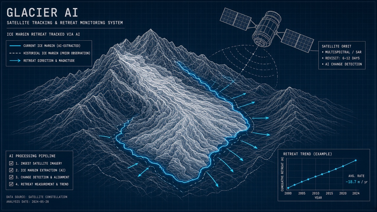
Alpine communities downstream of retreating glaciers watch lakes expand, moraines shift, and seasonal meltwater arrive earlier each decade. Scientists need consistent ice margin positions across thousands of glaciers, not just the handful accessible by foot survey each summer. Manual digitization of satellite scenes cannot keep pace with the rate of change or the volume of imagery streaming from Sentinel-2, Landsat, and commercial constellations. Glacier retreat AI satellite systems apply convolutional neural networks, vision transformers, and spatiotemporal models to segment ice, track calving fronts, and forecast how margins will move under changing climate forcing.
Hydropower operators, sea-level rise modelers, and mountain hazard teams depend on glacier inventories updated faster than annual field campaigns allow. Developers routing hazard alerts through AI chatbot dashboards should know whether ice extent comes from a physics-based mass balance model or a deep learning segmentation layer. For more explainers on climate AI, browse the EliteAI.tools blog index.
What Glacier Retreat AI Satellite Means in Plain Language
Glacier retreat AI satellite is the application of machine learning to optical and radar satellite imagery to map ice boundaries, measure area change over time, and predict future glacier extent or calving front position. Traditional glaciologists traced ice margins by hand on false-color composites. Modern pipelines feed multispectral tiles into U-Net, ResNet, or vision transformer encoders that output pixel-wise ice masks, then aggregate masks into area time series and feed forecasting models.
Retreat rate matters for water resources: many tropical and high-mountain communities rely on glacier melt during dry seasons. Sea-level contributions come from ice lost to the ocean at tidewater termini. Hazard planners track proglacial lakes that grow behind unstable moraine dams. Satellite AI scales inventory updates from regional to global without requiring every glacier to be visited in person.
| Satellite source | Revisit / resolution | Glacier AI use |
|---|---|---|
| Sentinel-2 (optical) | 5-day (twin satellites); 10 m bands | Seasonal margin mapping, debris cover |
| Landsat (optical) | 16-day; 30 m (legacy archives) | Decadal retreat time series |
| Sentinel-1 (SAR) | 6-day; cloud-penetrating radar | Wet-season ice mapping, velocity |
How the Underlying Glacier AI Pipeline Works
A glacier retreat AI pipeline downloads satellite tiles, applies atmospheric correction, runs semantic segmentation to classify ice vs rock vs water vs snow, post-processes masks for topology, and optionally couples outputs to climate reanalysis for forecasting. Each stage introduces error budgets that compound in area-change statistics.
GlaViTU and global ice segmentation
GlaViTU, a vision transformer approach for glacier mapping, reports global intersection-over-union (IoU) above 0.85 on held-out test regions, demonstrating that transformer backbones can generalize across mountain ranges when trained on diverse ice-debris-snow mixtures. High IoU means predicted ice pixels overlap strongly with reference outlines. Global models reduce the need to retrain a separate U-Net for every catchment, though local debris-covered tongues still challenge any global weights.
GlacierCastAI and spatiotemporal forecasting
GlacierCastAI combines ResNet50 feature extraction with ConvLSTM temporal layers to forecast glacier outlines, achieving IoU of 0.337 on future frames while incorporating ERA5 climate reanalysis that improved forecast skill by 3.4% over imagery-only baselines. IoU of 0.337 on future segmentation is modest compared to static mapping IoU above 0.85, which reflects the difficulty of predicting where ice will remain years ahead. The ERA5 gain shows that coupling satellite AI with temperature and precipitation fields adds measurable value beyond pure computer vision extrapolation.
GlaSpectra and calving front forecasting
GlaSpectra targets tidewater glacier calving fronts, using spectral-temporal deep learning to forecast where ice cliffs will retreat along fjords, supporting navigation and hazard planning in Arctic and Antarctic margins. Calving fronts move abruptly compared to slow alpine thinning; models must capture iceberg calving events and seasonal advance-retreat cycles. Spectral channels help separate bare ice, melange, and open water at termini.
| Model | Architecture / input | Reported metric |
|---|---|---|
| GlaViTU | Vision transformer; multispectral tiles | Global IoU > 0.85 |
| GlacierCastAI | ResNet50 + ConvLSTM; ERA5 climate | Forecast IoU 0.337; +3.4% with ERA5 |
| GlaSpectra | Spectral-temporal deep learning | Calving front forecasting |
Typical workflow steps
- Define glacier outlines of interest (RGI inventory IDs or custom AOI polygons).
- Acquire cloud-free Sentinel-2 or SAR scenes for melt season windows.
- Run segmentation model (GlaViTU or regional fine-tuned U-Net).
- Post-process: remove small holes, enforce hydrological consistency, compare to DEM.
- Compute area, length, and centerline retreat rates year over year.
- Optionally feed time series plus ERA5 into GlacierCastAI-class forecasters.
- Validate against ICESat-2 elevation change or field GPS stakes on subset.
Coupling Mass Balance Models and AI Outlines
Area change from segmentation models feeds mass balance frameworks that combine ice thickness estimates, surface melt models, and calving flux to project runoff and sea-level contribution. AI outlines reduce the labor of updating glacier polygons each season, but thickness change still depends on DEM differencing, gravimetry, or regional climate models. Teams should treat GlaViTU masks as dynamic boundaries inside physics models rather than standalone retreat predictions.
GlacierCastAI demonstrates the next step: forecasting where boundaries will move using ConvLSTM memory over historical masks plus ERA5 temperature and precipitation. Even with only IoU 0.337 on future frames, coupled workflows help water managers bracket plausible lake expansion behind moraine dams. Hydropower operators in the Andes and Himalaya use scenario ensembles: pessimistic retreat from AI forecast, central estimate from glaciological models, optimistic from slowed warming pathways.
Real Deployments and Published Evidence
Global glacier inventories from Randolph Glacier Inventory and regional centers increasingly incorporate automated outline updates between full manual revisions, driven by open satellite archives and pretrained segmentation weights. National hydrology services in Peru, Nepal, and Switzerland blend satellite-derived area change with stake measurements for water resource forecasts.
GlaViTU-level IoU above 0.85 supports operational mapping for clean ice surfaces. Debris-covered glaciers in the Himalaya and Andes remain harder: rock on ice mimics spectral signatures and confuses classifiers trained on cleaner Alpine ice. Teams publish separate accuracy tables for debris-covered subsets rather than reporting global IoU alone.
Forecasting models like GlacierCastAI sit earlier on the maturity curve. IoU of 0.337 on future masks signals that decadal planning should treat AI forecasts as scenario inputs coupled with mass balance models, not as standalone predictions. The 3.4% improvement from ERA5 argues for always fusing climate reanalysis with imagery features when building retreat projections. GlaSpectra-style calving front tools matter most for maritime glaciers where iceberg flux dominates mass loss rather than surface melt alone.
Limits, Risks, and Uncertainty
Glacier retreat AI can misclassify seasonal snow as perennial ice, underestimate debris-covered area, and propagate segmentation noise into exaggerated retreat rates when post-processing is weak. Cloud cover gaps create irregular time series that statistical models may misinterpret as acceleration.
- Seasonal snow confusion: Late-summer scenes best separate firn from fresh snow; spring maps bias high.
- Debris cover: Global IoU metrics often exclude hardest glaciers; local validation is mandatory.
- Forecast humility: Low future IoU means ensemble with physics models, not single AI output.
- Resolution limits: 10 m pixels miss narrow outlet glaciers affecting specific communities.
Who Should Use This and Who Should Wait
Regional water agencies, glacier hazard offices, and climate research groups with GIS capacity should deploy GlaViTU-class segmentation for seasonal inventory updates now, validating on local debris-covered glaciers. Communities needing legally defensible hazard zoning should combine AI outlines with field bathymetry and not rely on forecast IoU of 0.337 alone.
| Audience | Recommendation | Caveat |
|---|---|---|
| National hydrology service | Automate seasonal area from Sentinel-2 | Calibrate debris-covered tongues locally |
| Sea-level research consortium | Use GlaSpectra-class calving front tools | Pair with ice thickness models |
| Mountain community planner | Monitor proglacial lake growth annually | Field bathymetry for dam stability |
| Decadal infrastructure investor | Use forecast models as scenario input | Forecast IoU remains limited |
Frequently Asked Questions
How accurate is GlaViTU for global glacier mapping?
GlaViTU reports global IoU above 0.85 on test regions, indicating strong overlap between predicted and reference ice masks for many clean ice glaciers. Debris-covered and small glaciers may score lower; validate locally.
Why does GlacierCastAI use ERA5 climate data?
ERA5 reanalysis supplies temperature and precipitation fields that improved GlacierCastAI forecast IoU by 3.4% over imagery-only models, linking ice retreat to climate forcing. Climate fusion is recommended for any forecasting pipeline.
Why is forecast IoU much lower than mapping IoU?
Predicting future ice outlines (GlacierCastAI IoU 0.337) is harder than classifying present imagery (GlaViTU IoU > 0.85) because calving events and melt variability introduce irreducible uncertainty. Use forecasts as scenarios, not deterministic truth.
What does GlaSpectra add for tidewater glaciers?
GlaSpectra forecasts calving front position using spectral-temporal deep learning, supporting navigation and hazard assessment where cliffs retreat into fjords. Tidewater dynamics differ from alpine thinning.
How often can Sentinel-2 update glacier outlines?
Twin Sentinel-2 satellites revisit most glaciers every five days, though cloud cover in maritime mountains may yield only a handful of clear scenes per melt season. SAR fills gaps when optical fails.
How should teams validate AI glacier maps?
Compare AI outlines to ICESat-2 elevation trends, historic manual inventories, and field GPS stakes on a stratified glacier subset each year. Report IoU separately for debris-covered classes.
Which open data feeds support glacier AI pipelines?
Copernicus Sentinel-2 and Sentinel-1 archives, NASA Landsat collections, ERA5 climate reanalysis, and Randolph Glacier Inventory outlines provide free inputs for GlaViTU and GlacierCastAI-class workflows. Commercial sub-meter imagery helps narrow outlet glaciers but is optional for regional inventories.
Conclusion
Glacier retreat AI satellite methods scale ice monitoring from manual digitization to global segmentation and emerging forecast systems. GlaViTU delivers IoU above 0.85 for mapping; GlacierCastAI couples ResNet50 and ConvLSTM with ERA5 for forward-looking outlines at IoU 0.337; GlaSpectra addresses calving front dynamics. Credible use demands local validation on debris-covered ice, fusion with climate reanalysis for forecasts, and transparent reporting of uncertainty. Satellite AI accelerates inventories; physics-based mass balance and field measurements still anchor decisions that affect downstream communities. Open Sentinel archives lower the cost barrier for universities and hydrology agencies to adopt GlaViTU-class segmentation tools without proprietary imagery contracts or manual digitization bottlenecks.